A ride-share platform like Uber or Lyft is a real-time two-sided marketplace: it must continuously ingest GPS streams from millions of drivers, match riders to drivers with low latency, and handle financial transactions across a global fleet — all at 150 million monthly active users and 15 million trips per day. The deceptively simple act of "hail a ride" hides a formidable distributed systems problem: you need a near-real-time geospatial index that can handle millions of concurrent moving objects, a matching algorithm that optimizes globally rather than greedily, a reliable state machine for the trip lifecycle, surge pricing that responds to supply-demand imbalances in seconds, and a payment pipeline that is financially correct without slowing down the booking experience.
- GPS pipeline = at-most-once — one lost 5-second packet is negligible; guaranteed delivery overhead not worth it for location data.
- In-memory index + Cassandra — in-memory spatial index for sub-millisecond matching lookups; Cassandra for durable location history, partitioned by city and product type.
- Bipartite graph matching — batch incoming requests and solve globally for minimum average pickup time, not greedy nearest-driver per request.
- Geohash / S2 cells for geo-indexing — encode lat/lng into hierarchical cells; query nearby drivers by looking up cells at the right precision level.
- Consistent hashing (Ringpop) — distributes driver location data evenly across nodes with automatic repartitioning.
- Trip state machine — explicit states (REQUESTED → ACCEPTED → EN_ROUTE → IN_TRIP → COMPLETED) prevent illegal transitions and make retries safe.
- Surge pricing via supply/demand ratio — computed per geohash cell every 60–120 s; multiplier caps prevent PR disasters.
- Async payment — payment deduction and driver payout are off the critical trip-completion path to avoid processing delays degrading the booking experience.
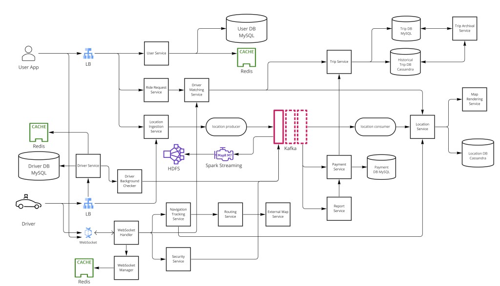
GPS packets flow every ~5s into a message queue (at-most-once delivery). An in-memory spatial index backed by Cassandra stores driver locations partitioned by city and product type. Matching uses batched bipartite graph optimization — not greedy nearest-driver — to minimize global average pickup time. Geohash or Google S2 cells enable O(1) radius queries. The trip is an explicit state machine. Surge pricing is a ratio computed per geohash cell. Payment is handled asynchronously via a third-party payment processor.
Step 1 — Clarify Requirements
Before diving in, scope the problem explicitly. Ride-share is broad — define exactly what you will and won't design.
Functional requirements
- Display available driver locations on a map in real time.
- Rider requests a trip — system matches them to a nearby available driver.
- ETA and upfront price estimate displayed before booking.
- Real-time location tracking during the trip (rider sees driver moving).
- Trip completion: fare calculation, payment, receipt.
- Driver earnings dashboard and trip history.
- Driver onboarding with background check.
Non-functional requirements
- Low latency — driver location updates visible within ~5 s; matching response under 2 s.
- High availability — the marketplace must be reachable even under partial failures; a down matching service means zero revenue.
- Consistency — a driver must not be double-matched; a trip must have exactly one driver.
- Global scale — 150 million monthly active users, 15 million trips per day across hundreds of cities.
- Geo-awareness — queries are inherently spatial; the system must index and search by location efficiently.
State out of scope explicitly: fraud detection, driver incentive programs, split fares, scheduled rides. This lets you focus the interview time on the genuinely hard parts — GPS pipeline, matching, and the trip state machine.
Step 2 — Capacity Estimation
Back-of-the-envelope math anchors your architecture choices. Assume the Uber scale: 150M MAU, 15M trips/day.
GPS write load
- Active drivers at peak: assume 1M concurrent drivers globally during evening rush.
- Each driver sends a GPS packet every 5 s → 1M ÷ 5 = 200,000 location writes/sec at peak.
- Each packet is ~100 bytes (driver_id, lat, lng, timestamp, heading) → ~20 MB/s of GPS ingestion.
- This is a bursty stream — a message queue is mandatory to absorb spikes.
Trip and matching load
- 15M trips/day ÷ 86,400 s ≈ ~174 trips/sec average; peak (Friday 6 pm) 3–5× → ~700 trip requests/sec.
- Each trip request triggers one matching computation, one ETA query, and at least two location reads (rider + drivers in radius).
- Matching is CPU-bound; plan for dedicated matching service instances, not shared with GPS ingestion.
Storage
- GPS history: 200K writes/sec × 100 bytes × 86,400 s ≈ ~1.7 TB of raw location data per day. Only the last known position needs to be in memory; history goes to Cassandra.
- Trip records: 15M trips × ~1 KB (trip metadata, fare, route summary) ≈ ~15 GB/day, totally manageable in SQL.
- In-memory spatial index: 1M concurrent drivers × 200 bytes per entry ≈ ~200 MB — trivially fits on a single node but is sharded for availability.
The GPS write load (200K/s) is the dominant data-plane concern. The trip request rate (700/s) is comparatively modest. Your architecture must handle the former without letting it starve the latter.
Step 3 — API Design
Key REST endpoints across the ride-share services:
# Driver — location update (high-frequency, at-most-once)
POST /driver/location
     { driver_id, lat, lng, heading, timestamp }

# Rider — request a trip
POST /trips
     { rider_id, pickup_lat, pickup_lng, dropoff_lat, dropoff_lng, product_type }
     → returns { trip_id, estimated_eta_s, estimated_fare, driver_info }

# Trip status (polled or WebSocket push)
GET  /trips/{trip_id}
     → { status, driver_location, eta_s, fare_cents }

# Driver — accept/decline a match
POST /trips/{trip_id}/accept   { driver_id }
POST /trips/{trip_id}/decline  { driver_id }

# Driver — trip lifecycle events
POST /trips/{trip_id}/arrived    # driver at pickup
POST /trips/{trip_id}/start      # trip begins
POST /trips/{trip_id}/complete   # trip ends, triggers fare + payment
The POST /driver/location endpoint is called at very high frequency and uses at-most-once delivery — the server accepts and moves on; no acknowledgement retry. The trip lifecycle endpoints are idempotent — calling /complete twice on an already-completed trip is a no-op at the state machine level.
Step 4 — Driver and Rider Registration
The User Service handles authentication and profile management for both sides of the marketplace. Driver onboarding involves an additional Background Checker that validates accident history, license validity, SSN, and vehicle status before a driver is activated. Frequently accessed user profiles are cached in Redis to reduce database load on high-traffic lookup paths.
Driver profiles carry additional state beyond what a rider profile needs: vehicle details (make, model, license plate, color), current availability status (OFFLINE / AVAILABLE / IN_TRIP), and product type eligibility (UberX, Comfort, Black, Pool). This eligibility is stored in SQL and cached; the matching service reads it to filter the driver pool before running the assignment algorithm.
Step 5 — GPS Ingestion Pipeline
Every active driver transmits a GPS packet approximately every 5 seconds, containing their user_id, current location, and a timestamp. At 15 million trips per day and assuming ~1M concurrent active drivers at peak, this produces ~200,000 writes per second — a high-volume, bursty write stream that a synchronous HTTP endpoint cannot absorb without being a bottleneck.
A message queue (Kafka or a purpose-built low-latency alternative) decouples the GPS producers from the location processing consumers, absorbing variability in QPS. Drivers write to the queue without waiting for confirmation; the consumers — the location update workers — drain the queue and update the in-memory spatial index and Cassandra asynchronously.
The delivery guarantee is at-most-once. A single lost GPS packet is acceptable because the next one arrives 5 seconds later — the cost of guaranteed delivery (retry loops, deduplication, higher latency) adds complexity for a negligible benefit. The contrast with payments is instructive: payment events use at-least-once because losing a payment message has real financial consequences.
GPS data pre-processing
Raw GPS readings are noisy — consumer-grade sensors have 3–5 m accuracy, and satellites occasionally produce wildly incorrect fixes. Before updating the spatial index, the location workers apply:
- Outlier rejection — discard readings that imply impossible speed (e.g., >200 km/h between two consecutive packets).
- Map matching — snap the lat/lng to the nearest road segment via the map service API, so the driver icon appears on the road rather than floating 10 m into a building.
- Kalman filtering (optional, higher fidelity) — smooth the GPS trace using a Kalman filter to reduce jitter on the rider's live-tracking map.
WebSockets maintain persistent connections — great for pushing data to clients, but 1M persistent inbound connections from driver apps would saturate connection table memory on a single gateway. The GPS write pattern (fire-and-forget every 5 s) is better served by short HTTP POSTs that a load balancer can distribute across stateless ingestion workers.
Step 6 — Geospatial Indexing
The core spatial operation is: "given a rider at (lat, lng), find all available drivers within radius R." Doing this efficiently at scale requires a purpose-built geospatial index rather than a brute-force scan of all driver records.
Geohash
Geohash encodes a (lat, lng) pair into a short alphanumeric string by recursively bisecting the world into a 2D grid. Each additional character halves the cell size. A 6-character geohash represents a ~1.2 km × 0.6 km cell. To find nearby drivers, you look up the target cell plus the 8 adjacent cells at the appropriate precision — nine lookups return all candidates within roughly 1–2 km.
-- Geohash precision table
length  cell width  cell height  use case
  4     ~39 km      ~20 km       city-level
  5     ~4.9 km     ~4.9 km      neighborhood
  6     ~1.2 km     ~0.61 km     block-level (good for driver search)
  7     ~153 m      ~153 m       fine-grained ETA

-- Finding nearby drivers: look up target cell + 8 neighbors
nearby_cells = geohash_neighbors(rider_geohash, precision=6)
-- returns 9 cells; query in-memory index for AVAILABLE drivers in those cells
Google S2 cells
Google S2 maps the sphere onto a cube, then uses a Hilbert curve to produce hierarchical cell IDs with excellent spatial locality. S2 cells at level 13 are roughly 1.3 km², similar to a 6-char geohash. S2 is what Uber uses internally (via their H3 library, a hexagonal variant); it handles polar distortions better than geohash and supports efficient cap/polygon queries. For an interview, either is acceptable — geohash is simpler to explain, S2/H3 is more production-correct.
QuadTree
A QuadTree recursively subdivides the 2D plane into four quadrants. Nodes that contain too many objects are split. QuadTrees adapt naturally to non-uniform distributions — dense urban cores get fine granularity, sparse rural areas stay coarse. The downside is that updates (a driver moving between cells) require tree restructuring, which is expensive compared to the hash-lookup approach of geohash. QuadTrees are more commonly seen in gaming spatial indexing than in ride-share production systems, but are a valid interview answer with the right caveats.
| Index Type | Strengths | Weaknesses |
|---|---|---|
| Geohash | Simple string prefix lookup; Redis native support; easy to shard by prefix | Cell boundary artifacts; non-uniform cell shapes at high latitudes |
| Google S2 / H3 | Uniform cell areas; excellent spatial locality; polygon/cap queries | More complex library; less widely understood |
| QuadTree | Adaptive to density; hierarchical aggregation | Expensive updates; complex tree balancing; in-memory only |
| R-Tree (PostGIS) | Mature SQL integration; handles polygons natively | SQL DB is too slow for 200K GPS writes/sec; not suitable for hot path |
Step 7 — Location Storage Architecture
Driver location data requires both high-speed lookup for matching and durable storage for trip history. These are two different access patterns that demand two different storage tiers:
| Layer | Technology | Purpose |
|---|---|---|
| Active index | In-memory search index | Sub-millisecond reads and writes for real-time driver lookup during matching |
| Persistent store | Cassandra (NoSQL) | Durable trip and location records; horizontally scalable writes |
| Partition key | DriverUUID + time bucket | Enables efficient time-range queries per driver |
| Sharding | City / segment / product type | Isolates load by market; UberX, UberPool, etc. have distinct supply pools |
| Distribution | Consistent hashing (Ringpop) | Distributes data evenly across worker nodes; auto-repartitioning via Airflow |
The in-memory index is partitioned by geohash prefix (or S2 cell ID prefix). Each shard is owned by a set of worker nodes determined by consistent hashing — Uber's Ringpop library implements this ring, allowing nodes to be added or removed without reshuffling all data. When a driver sends a location update, the ingestion worker hashes the driver's current geohash to find the owning shard, then updates that shard's in-memory map.
Cassandra is chosen for the persistent tier because it handles high write throughput with eventual consistency — the exact profile of GPS history. The partition key is (driver_id, date_hour_bucket) so all location records for a driver in a time window are co-located on one node, making "reconstruct this driver's route during trip X" a single partition read.
Step 8 — The Matching Algorithm
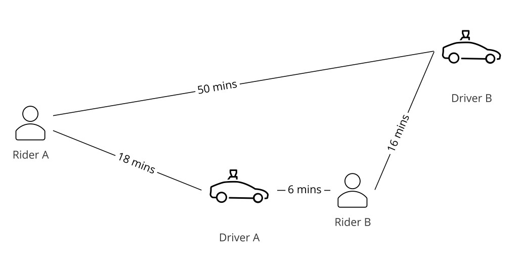
The intuitive approach — assign each incoming rider request to the nearest available driver — is greedy and globally suboptimal. If two riders are close to the same driver, the greedy approach gives the driver to the first requester, potentially leaving the second rider stranded with a much farther driver.
The correct framing is a bipartite graph matching problem: riders on one side, available drivers on the other, with edge weights representing pickup time. The system batches incoming requests within a short window and solves for the assignment that minimizes global average pickup time across all riders in the batch — not just the first rider in queue.
-- Greedy (suboptimal):
rider_A → nearest driver D1  (2 min)
rider_B → next driver D2     (8 min)
avg pickup = 5 min

-- Bipartite matching (optimal):
rider_A → driver D2          (4 min)
rider_B → driver D1          (4 min)
avg pickup = 4 min

-- Algorithm: Hungarian algorithm or min-cost flow
-- Batch window: typically 2–5 seconds
-- Edge weights: ETA from routing API (not Euclidean distance)
Matching pipeline in detail
- Geo lookup — query the in-memory spatial index for all
AVAILABLEdrivers within a search radius (e.g., 3 km) of the rider's pickup point. Filter by product type (UberX, Comfort, etc.). - ETA scoring — for each candidate driver, call the routing service (or use a lightweight straight-line estimate with a road factor) to get a realistic pickup ETA. Actual road ETA beats Euclidean distance significantly in grid-heavy cities like Manhattan.
- Batch solve — collect all pending rider requests in the current batch window. Build the bipartite graph with ETA as edge weights. Solve using the Hungarian algorithm (O(n³)) or a min-cost flow approximation for large batches.
- Offer dispatch — send a match offer to the assigned driver. If the driver declines or doesn't respond within ~15 s, the rider is re-queued for the next batch. Drivers who repeatedly decline are deprioritized in future batches.
- Lock the driver — once a driver accepts, atomically flip their status from
AVAILABLEtoIN_TRIPin the spatial index to prevent double-matching.
A driver 0.5 km away on the wrong side of a river may take 15 minutes; a driver 1.5 km away with a clear road takes 3 minutes. Using straight-line distance as the edge weight produces systematically wrong matches in real cities. Routing API calls are expensive — cache frequent city pairs or use pre-computed road factor heuristics for the scoring phase, then confirm with a full routing call after a match is found.
Step 9 — Trip State Machine
A trip is best modeled as an explicit state machine. Each state transition is triggered by an event — from driver or rider app, or from an internal timeout — and must be idempotent so that replaying a network-retried event does not advance the state incorrectly.
REQUESTED
  │ match found (bipartite algorithm)
  ▼
DRIVER_ASSIGNED
  │ driver accepts
  ▼
DRIVER_EN_ROUTE         ← driver heading to pickup
  │ driver arrives
  ▼
DRIVER_ARRIVED          ← driver waiting at pickup
  │ rider enters vehicle / driver taps "start"
  ▼
IN_TRIP                 ← ride in progress
  │ driver taps "complete" at destination
  ▼
COMPLETED               ← fare computed, payment triggered

  From any pre-COMPLETED state:
  REQUESTED / DRIVER_ASSIGNED → CANCELLED_BY_RIDER / NO_DRIVER_FOUND
  DRIVER_EN_ROUTE / DRIVER_ARRIVED → CANCELLED_BY_DRIVER / CANCELLED_BY_RIDER
Storing the state in a SQL row guarded by an application-level transition check prevents illegal hops (e.g., moving directly from REQUESTED to IN_TRIP). Each transition also publishes an event to Kafka so that downstream services — notification service (send "driver arriving" push), analytics service (record event), payment service (trigger charge on COMPLETED) — can react without being coupled to the trip service directly.
Timeout handling
- If a driver does not accept within ~15 s of being offered a match, the trip service re-queues the rider and marks the driver as deprioritized for the next matching cycle.
- If no driver is found after N retries over ~2 min, the trip moves to
NO_DRIVER_FOUNDand the rider is notified to try again later. - A distributed scheduler (e.g., Celery beat or a simple Kafka delayed message) drives these timeout transitions without a polling loop on the hot database.
Step 10 — ETA and Routing
Rather than building a proprietary mapping stack, ride-share platforms partner with external map providers (Google Maps, MapBox, OpenStreetMap) for road graph data, routing, and ETA calculation. A critical challenge is that GPS coordinates have no concept of roads — raw latitude/longitude must be snapped to the nearest road segment via map-matching before displaying a vehicle icon on-screen or computing ETA.
ETA computation layers
- Road graph — a weighted directed graph where nodes are road intersections and edges are road segments with travel-time weights derived from historical speed data and real-time traffic.
- Dijkstra / A* — shortest-path algorithms over the road graph; A* uses a geographic heuristic to prune the search space and run faster than Dijkstra in practice.
- Traffic adjustment — real-time traffic feeds (Google Traffic, HERE) modulate edge weights continuously; a road that takes 2 min at noon may take 12 min at 5 pm.
- ETA caching — popular city-pair ETAs are cached with short TTLs (30–60 s) since traffic changes frequently. Exact per-driver ETAs are computed fresh but use the cached road graph.
The matching service uses a lightweight ETA approximation (straight-line distance × road factor) for the scoring phase to avoid N routing API calls per batch. Once a match is confirmed, the full routing API computes the accurate ETA shown to the rider.
Step 11 — Surge Pricing
When demand exceeds supply in a geographic area, surge pricing raises fares to attract more drivers to the area and reduce demand from price-sensitive riders, rebalancing the market. Implementing surge pricing is a real-time data pipeline problem:
Computing the surge multiplier
- Every 60–120 seconds, the pricing service reads from the spatial index: for each geohash cell at precision 5–6 (neighborhood level), count
pending_requests(riders waiting) andavailable_drivers(AVAILABLE status). - Compute the supply/demand ratio:
ratio = pending_requests / max(available_drivers, 1). - Map the ratio to a multiplier via a lookup table (e.g., ratio < 0.5 → 1.0×; 0.5–1.0 → 1.2×; 1.0–2.0 → 1.5×; >2.0 → 2.0×). Cap the multiplier (e.g., 3.0×) to avoid PR disasters during emergencies.
- Write the multiplier to a Redis key per geohash cell with a short TTL (120 s). All pricing lookups hit Redis, not the spatial index.
What happens at geohash cell borders? A rider near the edge of a high-surge cell might be a few meters from a zero-surge cell. The system should aggregate multipliers from the rider's cell plus neighbors and take the weighted average, or simply use the rider's cell. The exact boundary behavior is a product policy decision — disclose surge clearly to riders regardless.
Upfront fare estimation
The fare shown before the rider books is an estimate based on: base_fare + (distance_km × per_km_rate + duration_min × per_min_rate) × surge_multiplier. The final fare uses actual GPS-tracked distance and time. If the actual fare significantly exceeds the estimate (e.g., detour by driver), rider protections cap the overage.
Step 12 — Map Services
Map services provide three critical functions: road graph data for routing, ETA computation, and the map tiles displayed in the app UI. Ride-share platforms partner with external providers rather than build these in-house — the investment required to maintain a global road graph (OpenStreetMap editing, traffic data partnerships, map rendering pipeline) is enormous and not a core competency.
Key integration points:
- Geocoding / reverse geocoding — convert human-readable addresses ("Pier 39, San Francisco") to (lat, lng) and back. Used for pickup/dropoff entry in the rider app.
- Directions API — given origin and destination, return turn-by-turn directions and ETA. Called once per confirmed match to show the driver their navigation route.
- Map matching API — snap raw GPS traces to road segments. Called by the GPS pre-processing pipeline and by the map display layer to show a smooth driver icon.
- Map tiles — raster or vector tiles for the app background map. Served via CDN from the map provider; the ride-share app does not re-host tiles.
Step 13 — Data Model
Key tables stored in SQL (trip records, user accounts) and in Cassandra (location history):
CREATE TABLE trips (
  id              BIGINT PRIMARY KEY,
  rider_id        BIGINT NOT NULL,
  driver_id       BIGINT,
  status          VARCHAR(32),   -- REQUESTED|DRIVER_ASSIGNED|...
  pickup_lat      DECIMAL(9,6),
  pickup_lng      DECIMAL(9,6),
  dropoff_lat     DECIMAL(9,6),
  dropoff_lng     DECIMAL(9,6),
  product_type    VARCHAR(16),   -- UBERX|COMFORT|BLACK|POOL
  surge_multiplier DECIMAL(4,2),
  estimated_fare_cents INT,
  actual_fare_cents    INT,
  requested_at    TIMESTAMP,
  completed_at    TIMESTAMP
);

CREATE TABLE drivers (
  id              BIGINT PRIMARY KEY,
  availability    VARCHAR(16),  -- OFFLINE|AVAILABLE|IN_TRIP
  product_types   TEXT,          -- comma-separated eligible types
  vehicle_plate   VARCHAR(16),
  rating          DECIMAL(3,2),
  last_lat        DECIMAL(9,6),
  last_lng        DECIMAL(9,6),
  last_geohash    VARCHAR(12),
  updated_at      TIMESTAMP
);-- GPS location history (write-heavy, time-series)
CREATE TABLE driver_location_history (
driver_id UUID,
time_bucket TEXT, -- e.g. '2024-05-24-18' (hourly bucket)
recorded_at TIMESTAMP,
lat DOUBLE,
lng DOUBLE,
heading SMALLINT,
PRIMARY KEY ((driver_id, time_bucket), recorded_at)
) WITH CLUSTERING ORDER BY (recorded_at DESC);
-- Partition = one driver × one hour; query = "all GPS for driver D in hour H"Step 14 — Payment Processing
Three architectural options exist for payment:
- Proprietary payment system — full control, high build cost and regulatory burden (PCI-DSS Level 1).
- Direct third-party integration (PayPal, Block/Square) — simpler, but tied to one provider.
- Unbranded payment gateway via processor partner — Uber's initial approach with Braintree; enables multi-provider flexibility and regional payment processor support without exposing the payment brand.
Payment deductions and driver payout calculations are handled asynchronously to keep them off the critical trip-completion path. When a trip reaches COMPLETED, the trip service publishes a TripCompleted event to Kafka. The payment service consumes this event, computes the final fare (actual distance × actual duration × surge multiplier), charges the rider's saved payment method via the processor API, and triggers driver payout (typically daily batch settlement rather than per-trip to reduce transfer fees).
Payment idempotency
The payment service passes a unique idempotency key (e.g., trip_id + "charge") to the payment processor on every charge call. If the network drops after the charge succeeds but before the response arrives, the retry with the same key is a no-op at the processor — the rider is not double-charged. A webhook from the processor confirms success or failure, which updates the trip record's payment status. A nightly reconciliation job catches any discrepancies between trip records and processor settlements.
What if the TripCompleted Kafka event is delivered twice (at-least-once semantics)? The payment service must dedup on trip_id — if a charge record already exists for the trip, skip the charge and return the existing result. This is the idempotent consumer pattern: every event consumer must handle re-delivery without side effects.
Step 15 — Scaling and Fault Tolerance
A global ride-share platform must survive regional outages, handle millions of concurrent connections, and route traffic intelligently across a distributed fleet of services.
Sharding the location index
The in-memory spatial index is sharded by city and product type — UberX in San Francisco is a completely separate data set from Comfort in London. Within a city, consistent hashing (Ringpop) distributes geohash prefixes across worker nodes. A driver moving between geohash cells triggers a location update that the hash ring routes to the correct shard automatically. When a node is added or removed, only the keys on the affected arc of the ring are remapped — minimizing data movement compared to naive modulo partitioning.
Multi-region deployment
Each major metro area runs its own matching, GPS ingestion, and spatial index cluster — a rider in Chicago never needs data from London. Cross-region communication is limited to user profile reads (cached aggressively) and global analytics pipelines. This geographic isolation keeps latency low, failure blast radius small, and regulatory data-residency requirements satisfied.
Circuit breakers and graceful degradation
- If the routing API (Google Maps) is slow, the matching service falls back to Euclidean-distance estimates. Matches are slightly less accurate but still dispatched.
- If the surge pricing service is down, fall back to a cached multiplier (or 1.0× as a safe default). Trips continue; pricing accuracy degrades temporarily.
- If Cassandra is unavailable, the GPS pipeline buffers in Kafka and catches up when the store recovers. Only the historical record is delayed — the in-memory index is unaffected.
WebSocket for real-time tracking
During an active trip, the rider's app displays the driver's position moving in real time. This requires a push channel, not polling — polling at 1 s intervals from millions of active trips would generate ~millions of HTTP requests per second for position data. The solution:
- A WebSocket gateway maintains persistent connections to active rider and driver apps.
- When the GPS pipeline processes a location update for a driver currently in trip, it publishes the new position to a per-trip Pub/Sub channel.
- The WebSocket gateway subscribes to that channel and pushes the update to the rider's connection.
- The gateway is stateless except for the connection table; it can be horizontally scaled behind a load balancer that supports sticky sessions (or a distributed pub/sub mesh like Redis Pub/Sub).
Step 16 — Key Tradeoffs
| Decision | Choice | Trade-off accepted |
|---|---|---|
| GPS delivery guarantee | At-most-once | Occasional missed packets; next update arrives in 5 s — negligible impact |
| Spatial index | In-memory + geohash | Memory cost; must be replicated; not durable — but speed is paramount for matching |
| Matching algorithm | Bipartite batch solve | Introduces 2–5 s batch window latency; globally better outcomes vs. greedy |
| Location persistence | Cassandra (eventual) | History is eventually consistent — acceptable; correctness needed for trip records (SQL) |
| Payment | Async (Kafka + processor) | Payment confirmed after trip; rare failure requires reconciliation job to catch |
| Map services | External provider | Cost per API call; dependency risk — but avoids enormous proprietary mapping investment |
| Surge computation | Periodic batch (60–120 s) | Up to 2-min lag on multiplier updates; acceptable given human decision timescales |
Ride-share design is dominated by two insights: GPS is a high-volume time-series stream (at-most-once, message queue + in-memory geohash index), and matching is a global optimization problem (bipartite graph), not a per-request greedy lookup. The trip state machine keeps lifecycle transitions correct and idempotent. Surge pricing is a periodic batch computation per geohash cell. Payment is intentionally async to keep it off the critical path. Everything else — consistent hashing, Cassandra, multi-region isolation — follows from handling those constraints at 200K GPS writes per second.
Why bipartite graph matching instead of greedy nearest-driver? Greedy assigns each rider to their nearest driver independently, which is locally optimal but globally suboptimal — it can leave nearby riders with much farther drivers. Batching requests and solving the bipartite assignment minimizes average pickup time across all riders.
Why at-most-once for GPS vs. at-least-once for payments? A dropped GPS packet has negligible impact (next arrives in 5 s); a dropped payment event has real financial consequences. Delivery guarantees should match the business cost of a lost message.
Why partition driver location data by city and product type? UberX and UberPool draw from separate driver pools; cross-city supply is irrelevant. Partitioning isolates load by market and makes matching queries fast within each segment.
How do you prevent a driver from being double-matched? The matching service atomically flips the driver's status from AVAILABLE to IN_TRIP in the spatial index before sending the offer. Any concurrent match attempt reads the updated status and skips that driver.
How does the surge multiplier get computed? Every 60–120 s, count pending_requests and available_drivers per geohash cell; compute their ratio; map to a multiplier table; write to Redis with a short TTL. Pricing reads are Redis hits — never a direct spatial index query.